Statistical Analysis and Graphing

Main Contents »

The subject of this chapter is the statistical analysis of data using Tcl. For this we use a dataset of meteorological data extracted from the website of the Royal Dutch Meteorological Institute, KNMI. The data are the daily amounts of precipitation in the period January 2003-June 2014 for a location in the centre of the Netherlands, De Bilt.

1. Introduction

For convenience, the data were extracted from the original files and put into a single file for further analysis (overview_day.txt). Each line contains the year and month and the daily precipitation. Zero precipitation is represented by a dot (.), which is not recognised by Tcl as a valid number:

string is double .
==> 0

Transforming "." to "0.0" is therefore part of reading the data:

set infile [open "overview_day.txt"]
#
# Read the file line by line and append the values
#
set data {}
while { [gets $infile line] > 0 } {
    foreach value [lrange $line 2 end] {
        if { $value eq "." } {
            set value 0.0
        }
        lappend data $value
    }
}
#
# We're done with the file
#
close $infile

We now have all the data in one long list. This is a convenient form for the kind of analysis we want to perform.

2. A simple graph

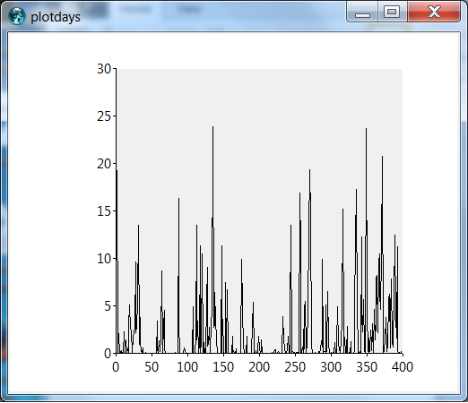
One of the first things you can do with the data just read is create a plot to get an impression:

#
# Load the Plotchart package for drawing the plots
#
package require Plotchart
#
# Create the plot
#
pack [canvas .c -width 500 -height 400]
set p [::Plotchart::createXYPlot .c {0 400 50} {0 30 5}]

for {set i 0} {$i < 400} {incr i} {
    $p plot data $i [lindex $data $i]
}

The graph shows a very spiky timeseries - mostly low values and short peaks. This is typical for precipitation data.

rain_per_day

3. Distribution of the data

The most basic analysis we can do is determining such parameters as the mean value, the minimum and the maximum:

#
# Get the statistics package - part of Tcllib
#
package require math::statistics
#
puts "Mean:\t[::math::statistics::mean $data]"
puts "Minimum:\t[::math::statistics::min $data]"
puts "Minimum:\t[::math::statistics::max $data]"
puts "St.dev:\t[::math::statistics::stdev $data]"

The result:

Mean:   2.476959325396846
Minimum:        0.0
Minimum:        61.6
St.dev: 5.0592335965823185

These numbers do not give much insight in the distribution - the amount of precipitation is not a Gaussian stochastic. So to gain more insight, let us determine a histogram of the precipitation data: How many values smaller than 1, in the range 1-2, 2-5, 5-10, 10-20, 20-30, 30-40 and 40-50, more than 50 mm?

set limits {1.0 2.0 5.0 10.0 20.0 30.0 40.0 50.0}
foreach limit  [concat $limits >50] \
        number [::math::statistics::histogram $limits $data] {
    puts "$limit\t$number"
}

which produces:

1.0     2604
2.0     274
5.0     491
10.0    377
20.0    223
30.0    43
40.0    13
50.0    4
>50     3

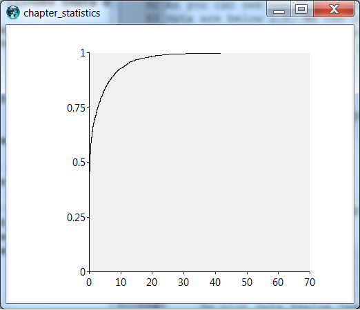
As you can see the distribution is very skewed: more than half the data are below 1.0. We can refine the limits of the histogram, we can also draw the cumulative distribution by sorting the values and using the index as the y-value or perhaps better, the index scaled with the number of data:

package require Plotchart
#
pack [canvas .c -width 500 -height 400]
set p [::Plotchart::createXYPlot .c {0 70 10} {0 1 0.25}]
#
# Draw the data
#
set scale [llength $data]
set y     0
foreach value [lsort -real -increasing $data] {
    $p plot data $value [expr {$y / double($scale)}]
    incr y
}

The graph below shows that the data are really concentrated around the zero value. During roughly one half of the days in the period we are examining there was no precipitation or very little. This has consequences if you want to generate artificial precipitation data for modelling purposes. Such a precipitation generator would have to generate zero values during about half the days and on the other days the generated values should follow the skewed distribution.

4. Seasonal variation

There are at least two further questions we can ask about these data:

Is there any seasonal effect?
If it rains on day t, does it also rain on day t+1? Or if it is dry on day t, will it also be dry on day t+1?

Let us start with the first question. We are going to divide the data per month, determine the mean value and plot the results in a barchart:

First we store the data per month, via the arrays all_data and nonzero_data which store all precipitation data and only the non-zero data respectively (given the large amount of data with a very value):

set infile [open "overview_day.txt"]
#
# Read the file line by line and append the values
#
while { [gets $infile line] > 0 } {
    set month [lindex $line 1]
    foreach value [lrange $line 2 end] {
        if { $value eq "." } {
            set value 0.0
        } else {
            lappend nonzero_data($month) $value
        }
        lappend all_data($month) $value
    }
}
#
# We're done with the file
#
close $infile

The we calculate the mean values per month and draw the results as a barchart:

set months {01 02 03 04 05 06 07 08 09 10 11 12}
#
package require Plotchart
package require math::statistics
#
pack [canvas .c -width 500 -height 400]
set p [::Plotchart::createBarchart .c $months {0.0 6.0 2.0} 2]
#
set all_means     {}
set nonzero_means {}
foreach month $months {
    lappend all_means     [::math::statistics::mean $all_data($month)]
    lappend nonzero_means [::math::statistics::mean $nonzero_data($month)]
}
#
$p plot alldata $all_means     lime
$p plot nonzero $nonzero_means red
#
$p legendconfig -position top-left
$p legend alldata "All data"
$p legend nonzero "Only non-zero"

The months are used as a label, not as a numeric index.

The barchart looks like this:

season

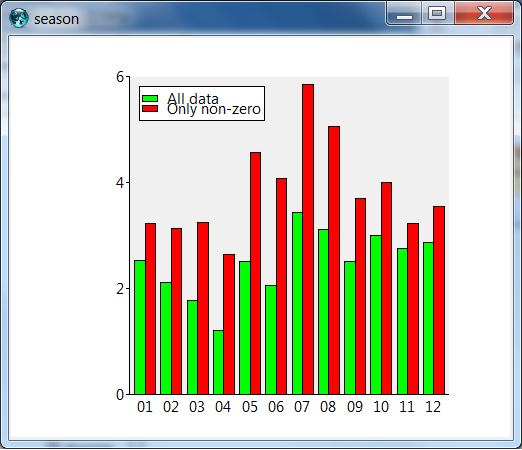
There seems to be only a very weak seasonal variation and actually the data show that the summer months are the wettest, though precipitation may be expected throughout the year.

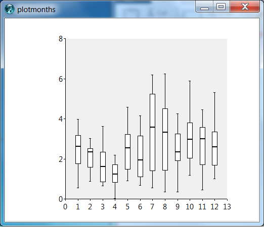
The graph does not tell us much about the variation from year to year, though. If we consider instead the individual months and create box-andwhisker plots, we can see how variable the precipitation actually is:

package require Plotchart
#
# Store the mean precipitation per month
#
set infile [open "overview_day.txt"]
#
while { [gets $infile line] > 0 } {
    scan [lindex $line 1] %d month ;# Avoid problems with leading zero!
    set sum   0.0
    set count 0
    foreach value [lrange $line 2 end] {
        incr count
        if { $value ne "." } {
            set sum [expr {$sum + $value}]
        }
    }
    lappend month_data($month) [expr {$sum/$count}]
}
close $infile
#
pack [canvas .c -width 500 -height 400]
set p [::Plotchart::createXYPlot .c {0 13 1} {0.0 8.0 2.0}]
#
for {set month 1} {$month <= 12} {incr month} {
    $p box-and-whiskers month $month $month_data($month)
}

The resulting plot reveals that the rainfall has very little consistency, as the 25% and 75% percentiles typically are half and 1.5 times the mean. Especially in the summer months, the amount of rain varies enormously.

whiskers

Strings that start with a zero are interpreted as an octal number by the expr command. That means that a string like "08" causes a problem when used in a numerical context. It is a remnant from the "old days", when octals played a much larger role than they do nowadays. One solution to this problem is to use the scan command to convert the string to a number first, as done in the above code.

5. Will it rain tomorrow?

The second question, whether a wet day means the next day will be wet as well requires a very different approach. It boils down to determining the correlation between the precipitation data for subsequent days. But rather than looking at the actual amount we want to know the chance that tomorrow will be wet if today was wet. Let us define a wet day as a day that the precipitation is larger than 0.1 (this seems to be the measurement threshold). Now we need to count the number of wet days and the number of pairs of wet days:

set number_wet 0
set wet_dry    {}
foreach v $data {
    if { $value eq "." || $value <= 0.1} {
        set value 0
    } else {
        incr number_wet
        set value 1
    }
    lappend wet_dry $value
}

This code fragment gives us an array of wet/dry indicators rather than the precipitation data themselves.

We create two extended lists of data, a copy shifted by a single day and an extra value at the beginning or the end to make the counting easier:

set shifted_wet_dry [concat 0 $wet_dry]
set wet_dry         [concat $wet_dry 0]

Now we can count how many times two consecutive days are wet: set pairs 0

foreach v1 $data v2 $shifted_data {
    set pairs [expr {$pairs + $v1 * $v2}]
}

puts "Total number of data: [llength $wet_dry]"
puts "Number of wet days:   $number_wet"
puts "Pairs of wet days:    $pairs"

And the result is remarkably clear:

Total number of data: 4033
Number of wet days:   2178
Pairs of wet days:    1544

So it is quite probable that a wet day is followed by another wet day. We do not really need to determine the probability that this is just a coincidence. Or do we? Let us do the formal analysis anyway:

If there is no correlation between two consecutive days, then the series would be binomially distributed. The probability of getting a "1" from this distribution is p = 2178/4033 = 0.54.
The 2178 wet days would be followed by 2178*p = 1176 other wet days in this case. If the distribution is really binomial, then the standard deviation would be: sqrt(4033*p*(1-p)) = 31.7.
Since we have 1544 pairs instead of 1176, the deviation from the mean is about ten times the standard deviation.
Unfortunately, we can not simply use the binomial distribution and determine the probability that such a deviation occurs: we are looking for two properties of the same timeseries. There are so many wet days that they can just clutter up even if they are independent.
Instead we need to construct new timeseries based on the assumption of a binomial distribution and count the number of pairs of wet days. From the histogram of these counts we can then determine if 1544 pairs are improbable for a binomial distribution or not.

Here is code to generate these series and determine the probability we seek:

package require math::statistics
#
set number_data 4033
set p           [expr {2178/double($number_data)}]
#
set counts {}
for {set i 0} {$i < 1000} {incr i} {
    set previous    0
    set count_pairs 0
    for {set j 0} {$j < 4033} {incr j} {
        set current [expr {rand() <= $p}]

        if { $previous && $current } {
            incr count_pairs
        }
        set previous $current
    }
    lappend counts $count_pairs
}
#
set limits {1000 1100 1200 1300 1400 1500 1600 1700 1800 1900 2000}
puts "Distribution:"
#
foreach limit [concat $limits >2000] count [::math::statistics::histogram $limits $counts] {
    puts "$limit:\t$count"
}

From the output of this program we can see that 1544 pairs of wet days are very improbable for a binomial distribution with parameter p=0.54:

Distribution:
1000:   0
1100:   23
1200:   692
1300:   285
1400:   0
1500:   0
1600:   0
1700:   0
1800:   0
1900:   0
2000:   0
>2000:  0

So in the one thousand simulations not a single one comes close to the number we found in the measurements. That is, rain on two consecutive days is no coincidence.